
The Probability Density Function (PDF) for a Gaussian (Normal) distribution describes the likelihood of a continuous random variable taking a specific value. It is characterized by its signature “bell curve” shape, which is symmetric around the mean.

K.K. Gan L3: Gaussian Probability Distribution 1
Lecture 3
Gaussian Probability Distribution
p(x) =
1
s
2
p
e
-
(x -
m
)
2
2
s
2
gaussian
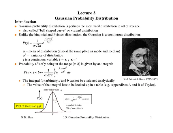
Plot of Gaussian pdf
x
P(x)
Introduction
l Gaussian probability distribution is perhaps the most used distribution in all of science.
u also called “bell shaped curve” or normal distribution
l Unlike the binomial and Poisson distribution, the Gaussian is a continuous distribution:
m
= mean of distribution (also at the same place as mode and median)
s
2
= variance of distribution
y is a continuous variable (-∞ £ y £ ∞)
l Probability (P) of y being in the range [a, b] is given by an integral:
u The integral for arbitrary a and b cannot be evaluated analytically
+ The value of the integral has to be looked up in a table (e.g. Appendixes A and B of Taylor).
†
P(y) =
1
s
2
p
e
-
(y-
m
)
2
2
s
2
†
P(a < y < b) =
1
s
2
p
e
-
(y-
m
)
2
2
s
2
a
b
Ú
dy
Karl Friedrich Gauss 1777-1855

K.K. Gan L3: Gaussian Probability Distribution 2
It is very unlikely (< 0.3%) that a
measurement taken at random from a
Gaussian pdf will be more than ± 3s
from the true mean of the distribution.
l The total area under the curve is normalized to one.
+ the probability integral:
l We often talk about a measurement being a certain number of standard deviations (
s
) away
from the mean (
m
) of the Gaussian.
+ We can associate a probability for a measurement to be |
m
- n
s
|
from the mean just by calculating the area outside of this region.
n
s
Prob. of exceeding ±n
s
0.67 0.5
1 0.32
2 0.05
3 0.003
4 0.00006
Relationship between Gaussian and Binomial distribution
l The Gaussian distribution can be derived from the binomial (or Poisson) assuming:
u p is finite
u N is very large
u we have a continuous variable rather than a discrete variable
l An example illustrating the small difference between the two distributions under the above conditions:
u Consider tossing a coin 10,000 time.
p(heads) = 0.5
N = 10,000
†
P(-• < y < •) =
1
s
2
p
e
-
(y-
m
)
2
2
s
2
-•
•
Ú
dy =1

K.K. Gan L3: Gaussian Probability Distribution 3
n For a binomial distribution:
mean number of heads =
m
= Np = 5000
standard deviation
s
= [Np(1 - p)]
1/2
= 50
+ The probability to be within ±1
s
for this binomial distribution is:
n For a Gaussian distribution:
+ Both distributions give about the same probability!
Central Limit Theorem
l Gaussian distribution is important because of the Central Limit Theorem
l A crude statement of the Central Limit Theorem:
u Things that are the result of the addition of lots of small effects tend to become Gaussian.
l A more exact statement:
u Let Y
1
, Y
2
,...Y
n
be an infinite sequence of independent random variables
each with the same probability distribution.
u Suppose that the mean (
m
) and variance (
s
2
) of this distribution are both finite.
+ For any numbers a and b:
+ C.L.T. tells us that under a wide range of circumstances the probability distribution
that describes the sum of random variables tends towards a Gaussian distribution
as the number of terms in the sum Æ∞.
†
P =
10
4
!
(10
4
- m)!m!
m=5000-50
5000+50
Â
0.5
m
0.5
10
4
-m
= 0.69
†
P(
m
-
s
< y <
m
+
s
) =
1
s
2
p
e
-
(y-
m
)
2
2
s
2
m
-
s
m
+
s
Ú
dy ª 0.68
†
lim
nƕ
P a <
Y
1
+Y
2
+...Y
n
- n
m
s
n
< b
È
Î
Í
˘
˚
˙
=
1
2
p
e
-
1
2
y
2
a
b
Ú
dy
Actually, the Y’s can
be from different pdf’s!


