This document is Lecture 3 on Gaussian Probability Distribution by K.K. Gan. It covers key concepts such as the Gaussian curve, Central Limit Theorem, and the relationship between Gaussian and Binomial distributions. The lecture is structured to provide a comprehensive understanding of probability distributions in a scientific context.

K.K. Gan L3: Gaussian Probability Distribution 1
Lecture 3
Gaussian Probability Distribution
p(x) =
1
s
2
p
e
-
(x -
m
)
2
2
s
2
gaussian
Plot of Gaussian pdf
x
P(x)
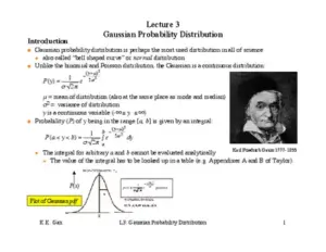
Introduction
l Gaussian probability distribution is perhaps the most used distribution in all of science.
u also called Òbell shaped curveÓ or normal distribution
l Unlike the binomial and Poisson distribution, the Gaussian is a continuous distribution:
m
= mean of distribution (also at the same place as mode and median)
s
2
= variance of distribution
y is a continuous variable (-! £ y £ !)
l Probability (P) of y being in the range [a, b] is given by an integral:
u The integral for arbitrary a and b cannot be evaluated analytically
+ The value of the integral has to be looked up in a table (e.g. Appendixes A and B of Taylor).
P(y) =
1
s
2
p
e
-
(y-
m
)
2
2
s
2
P(a < y < b) =
1
s
2
p
e
-
(y-
m
)
2
2
s
2
a
b
ò
dy
Karl Friedrich Gauss 1777-1855

K.K. Gan L3: Gaussian Probability Distribution 2
It is very unlikely (< 0.3%) that a
measurement taken at random from a
Gaussian pdf will be more than ± 3s
from the true mean of the distribution.
l The total area under the curve is normalized to one.
+ the probability integral:
l We often talk about a measurement being a certain number of standard deviations (
s
) away
from the mean (
m
) of the Gaussian.
+ We can associate a probability for a measurement to be |
m
- n
s
|
from the mean just by calculating the area
outside of this region.
n
s
Prob. of exceeding ±n
s
0.67 0.5
1 0.32
2 0.05
3 0.003
4 0.00006
Relationship between Gaussian and Binomial distribution
l The Gaussian distribution can be derived from the binomial (or Poisson) assuming:
u p is finite
u N is very large
u we have a continuous variable rather than a discrete variable
l An example illustrating the small difference between the two distributions under the above conditions:
u Consider tossing a coin 10,000 time.
p(heads) = 0.5
N = 10,000
P(-¥ < y < ¥) =
1
s
2
p
e
-
(y-
m
)
2
2
s
2
-¥
¥
ò
dy =1

K.K. Gan L3: Gaussian Probability Distribution 3
n For a binomial distribution:
mean number of heads =
m
= Np = 5000
standard deviation
s
= [Np(1 - p)]
1/2
= 50
+ The probability to be within ±1
s
for this binomial distribution is:
n For a Gaussian distribution:
+ Both distributions give about the same probability!
Central Limit Theorem
l Gaussian distribution is important because of the Central Limit Theorem
l A crude statement of the Central Limit Theorem:
u Things that are the result of the addition of lots of small effects tend to become Gaussian.
l A more exact statement:
u Let Y
1
, Y
2
,...Y
n
be an infinite sequence of independent random variables
each with the same probability distribution.
u Suppose that the mean (
m
) and variance (
s
2
) of this distribution are both finite.
+ For any numbers a and b:
+ C.L.T. tells us that under a wide range of circumstances the probability distribution
that describes the sum of random variables tends towards a Gaussian distribution
as the number of terms in the sum ®!.
P =
10
4
!
(10
4
- m)!m!
m=5000-50
5000+50
å
0.5
m
0.5
10
4
-m
= 0.69
P(
m
-
s
< y <
m
+
s
) =
1
s
2
p
e
-
(y-
m
)
2
2
s
2
m
-
s
m
+
s
ò
dy » 0.68
lim
n®¥
P a <
Y
1
+Y
2
+...Y
n
- n
m
s
n
< b
é
ë
ê
ù
û
ú
=
1
2
p
e
-
1
2
y
2
a
b
ò
dy
Actually, the YÕs can
be from different pdfÕs!