
For MATH 241: Calculus III at the University of Maryland (UMD), students often utilize formula sheets for quick reference on vectors, multivariable derivatives, and complex integration. While professors may provide specific sheets during exams, the following are standard resources and key formulas used in the course.
Derivatives
D
x
e
x
= e
x
D
x
sin(x)=cos(x)
D
x
cos(x)=sin(x)
D
x
tan(x)=sec
2
(x)
D
x
cot(x)=csc
2
(x)
D
x
sec(x)=sec(x)tan(x)
D
x
csc(x)=csc(x)cot(x)
D
x
sin
1
=
1
p
1x
2
,x 2 [1, 1]
D
x
cos
1
=
1
p
1x
2
,x 2 [1, 1]
D
x
tan
1
=
1
1+x
2
,
⇡
2
x
⇡
2
D
x
sec
1
=
1
|x|
p
x
2
1
, |x| > 1
D
x
sinh(x)=cosh(x)
D
x
cosh(x)=sinh(x)
D
x
tanh(x)=sech
2
(x)
D
x
coth(x)=csch
2
(x)
D
x
sech(x)=sech(x)tanh(x)
D
x
csch(x)=csch(x)coth(x)
D
x
sinh
1
=
1
p
x
2
+1
D
x
cosh
1
=
1
p
x
2
1
,x > 1
D
x
tanh
1
=
1
1x
2
1 <x<1
D
x
sech
1
=
1
x
p
1x
2
, 0 <x<1
D
x
ln(x)=
1
x
Integrals
R
1
x
dx = ln |x| + c
R
e
x
dx = e
x
+ c
R
a
x
dx =
1
ln a
a
x
+ c
R
e
ax
dx =
1
a
e
ax
+ c
R
1
p
1x
2
dx = sin
1
(x)+c
R
1
1+x
2
dx = tan
1
(x)+c
R
1
x
p
x
2
1
dx =sec
1
(x)+c
R
sinh(x)dx = cosh(x)+c
R
cosh(x)dx = sinh(x)+c
R
tanh(x)dx = ln |cosh(x)| + c
R
tanh(x)sech(x)dx = sech(x)+c
R
sech
2
(x)dx = tanh(x)+c
R
csch(x)coth(x)dx = csch(x)+c
R
tan(x)dx = ln |cos(x)| + c
R
cot(x)dx = ln |sin(x)| + c
R
cos(x)dx = sin(x)+c
R
sin(x)dx = cos(x)+c
R
1
p
a
2
u
2
dx = sin
1
(
u
a
)+c
R
1
a
2
+u
2
dx =
1
a
tan
1
u
a
+ c
R
ln(x)dx =(xln(x)) x + c
U-Substitution
Let u = f(x)(canbemorethanone
variable).
Determine: du =
f (x)
dx
dx and solve for
dx.
Then, if a definite integral, substitute
the bounds for u = f (x)ateachbounds
Solve the integral using u.
Integration by Parts
R
udv = uv
R
vdu
Fns and Identities
sin(cos
1
(x)) =
p
1 x
2
cos(sin
1
(x)) =
p
1 x
2
sec(tan
1
(x)) =
p
1+x
2
tan(sec
1
(x))
=(
p
x
2
1ifx 1)
=(
p
x
2
1 if x 1)
sinh
1
(x)=lnx +
p
x
2
+1
sinh
1
(x)=lnx +
p
x
2
1,x1
tanh
1
(x)=
1
2
ln x +
1+x
1x
, 1 <x<1
sech
1
(x)=ln[
1+
p
1x
2
x
], 0 <x1
sinh(x)=
e
x
e
x
2
cosh(x)=
e
x
+e
x
2
Trig Identities
sin
2
(x)+cos
2
(x)=1
1+tan
2
(x)=sec
2
(x)
1+cot
2
(x)=csc
2
(x)
sin(x ± y)=sin(x)cos(y) ± cos(x)sin(y)
cos(x ± y)=cos(x)cos(y) ± sin(x)sin(y)
tan(x ± y)=
tan(x)±tan(y)
1⌥tan(x) tan(y)
sin(2x)=2sin(x)cos(x)
cos(2x)=cos
2
(x) sin
2
(x)
cosh(n
2
x) sinh
2
x =1
1+tan
2
(x)=sec
2
(x)
1+cot
2
(x)=csc
2
(x)
sin
2
(x)=
1cos(2x)
2
cos
2
(x)=
1+cos(2x)
2
tan
2
(x)=
1cos(2x)
1+cos(2x)
sin(x)=sin(x)
cos(x)=cos(x)
tan(x)=tan(x)
Calculus 3 Concepts
Cartesian coords in 3D
given two p oints:
(x
1
,y
1
,z
1
)and(x
2
,y
2
,z
2
),
Distance between them:
p
(x
1
x
2
)
2
+(y
1
y
2
)
2
+(z
1
z
2
)
2
Midpoint:
(
x
1
+x
2
2
,
y
1
+y
2
2
,
z
1
+z
2
2
)
Sphere with center (h,k,l) and radius r:
(x h)
2
+(y k)
2
+(z l)
2
= r
2
Vector s
Vector : ~u
Unit Vector: ˆu
Magnitude: ||~u|| =
q
u
2
1
+ u
2
2
+ u
2
3
Unit Vector: ˆu =
~u
||~u||
Dot Product
~u · ~v
Produces a Scalar
(Geometrically, the dot product is a
vector pro jection)
~u =<u
1
,u
2
,u
3
>
~v =<v
1
,v
2
,v
3
>
~u · ~v =
~
0meansthetwovectorsare
Perpendicular ✓ is th e an gle between
them.
~u · ~v = ||~u|| ||~v|| cos(✓)
~u · ~v = u
1
v
1
+ u
2
v
2
+ u
3
v
3
NOTE:
ˆu · ˆv = cos(✓)
||~u||
2
= ~u · ~u
~u · ~v = 0 when ?
Angle Between ~u and ~v:
✓ = cos
1
(
~u·~v
||~u|| ||~v||
)
Pro jection of ~u onto ~v:
pr
~v
~u =(
~u·~v
||~v||
2
)~v
Cross Product
~u ⇥ ~v
Produces a Vector
(Geometrically, the cross product is the
area of a p aralellogram with sides ||~u||
and ||~v||)
~u =<u
1
,u
2
,u
3
>
~v =<v
1
,v
2
,v
3
>
~u ⇥ ~v =
ˆ
i
ˆ
j
ˆ
k
u
1
u
2
u
3
v
1
v
2
v
3
~u ⇥ ~v =
~
0meansthevectorsareparalell
Lines and Planes
Equation of a Plane
(x
0
,y
0
,z
0
) is a point on the plane and
<A,B,C>is a normal vector
A(x x
0
)+B(y y
0
)+C(z z
0
)=0
<A,B,C>· <xx
0
,yy
0
,zz
0
>=0
Ax + By + Cz = D where
D = Ax
0
+ By
0
+ Cz
0
Equation of a line
AlinerequiresaDirectionVector
~u =<u
1
,u
2
,u
3
> and a point
(x
1
,y
1
,z
1
)
then,
aparameterizationofalinecouldbe:
x = u
1
t + x
1
y = u
2
t + y
1
z = u
3
t + z
1
Distance from a Point to a Plane
The distance from a point (x
0
,y
0
,z
0
)to
a plane Ax+By+Cz=D can be expressed
by the formula:
d =
|Ax
0
+By
0
+Cz
0
D|
p
A
2
+B
2
+C
2
Coord Sys Conv
Cylindrical to Rectangular
x = r cos(✓)
y = r sin(✓)
z = z
Rectangular to Cylindrical
r =
p
x
2
+ y
2
tan(✓)=
y
x
z = z
Spherical to Rectangular
x = ⇢ sin()cos(✓)
y = ⇢ sin()sin(✓)
z = ⇢ cos()
Rectangular to Spherical
⇢ =
p
x
2
+ y
2
+ z
2
tan(✓)=
y
x
cos()=
z
p
x
2
+y
2
+z
2
Spherical to Cylindrical
r = ⇢ sin()
✓ = ✓
z = ⇢ cos()
Cylindrical to Spherical
⇢ =
p
r
2
+ z
2
✓ = ✓
cos()=
z
p
r
2
+z
2
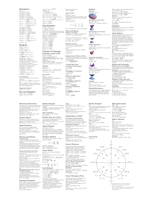
Surfaces
Ellipsoid
x
2
a
2
+
y
2
b
2
+
z
2
c
2
=1
Hyperboloid of One Sheet
x
2
a
2
+
y
2
b
2
z
2
c
2
=1
(Major Axis: z because it follows - )
Hyperboloid of Two Sheets
z
2
c
2
x
2
a
2
y
2
b
2
=1
(Major Axis: Z because it is the one not
subtracted)
Elliptic Paraboloid
z =
x
2
a
2
+
y
2
b
2
(Major Axis: z because it is the variable
NOT squared)
Hyperbolic Paraboloid
(Major Axis: Z axis because it is not
squared)
z =
y
2
b
2
x
2
a
2
Elliptic Cone
(Major Axis: Z axis because it’s the only
one being subtracted)
x
2
a
2
+
y
2
b
2
z
2
c
2
=0
Cylinder
1ofthevariablesismissing
OR
(x a)
2
+(y b
2
)=c
(Major Axis is missing variable)
Partial D er ivatives
Partial Derivatives are simply holding all
other variables constant (and act like
constants for the derivative) and only
taking the derivative with respect to a
given variable.
Given z=f(x,y), the partial derivative of
zwithrespecttoxis:
f
x
(x, y)=z
x
=
@z
@x
=
@f (x,y)
@x
likewise for partial with respect to y:
f
y
(x, y)=z
y
=
@z
@y
=
@f (x,y)
@y
Notation
For f
xyy
,work”insidetooutside”f
x
then f
xy
,thenf
xyy
f
xyy
=
@
3
f
@x@
2
y
,
For
@
3
f
@x@
2
y
,workrighttoleftinthe
denominator
Gradients
The Gradient of a function in 2 variables
is rf =<f
x
,f
y
>
The Gradient of a function in 3 variables
is rf =<f
x
,f
y
,f
z
>
Chain Rule(s)
Take the Par ti al der ivat ive wit h r es p ect
to the first-order variables of the
function times the partial (or normal)
derivative of the first-order variable to
the ultimate variable you are looking for
summed with the same process for other
first-order variables this makes sense for.
Example:
let x = x(s,t), y = y(t) and z = z (x,y).
zthenhasfirstpartialderivative:
@z
@x
and
@z
@y
xhasthepartialderivatives:
@x
@s
and
@x
@t
and y has the derivative:
dy
dt
In this case (with z containing x and y
as well as x and y b oth containing s and
t), the chain rule for
@z
@s
is
@z
@s
=
@z
@x
@x
@s
The chain rule for
@z
@t
is
@z
@t
=
@z
@x
@x
@t
+
@z
@y
dy
dt
Note: the use of ”d ” inste ad of ”@ ”with
the function of only one independent
variable
Limits and Continuity
Limits in 2 or more variables
Limits taken over a vectorized limit just
evaluate separately for each component
of the limit.
Strategies to show limit exists
1. Plug in Numbers, Everything is Fine
2. Algebraic Manipulation
-factoring/dividing out
-use trig identites
3. Change to polar coords
if(x, y) ! (0, 0) , r ! 0
Strategies to show limit DNE
1. Show limit is di↵erent if approached
from di↵erent paths
(x=y, x = y
2
, etc.)
2. Switch to Polar coords and show the
limit DNE.
Continunity
Afn,z = f (x, y), is continuous at (a,b)
if
f(a, b)=lim
(x,y)!(a,b)
f(x, y)
Which means:
1. The limit exists
2. The fn value is defined
3. They are the same value
Directional Derivatives
Let z=f(x,y) be a fuction, (a,b) ap point
in the domain (a valid input point) and
ˆu aunitvector(2D).
The Directional Derivative is then the
derivative at the point (a,b) in the
direction of ˆu or:
D
~u
f(a, b)= ˆu · rf(a, b)
This will return a scalar.4-Dversion:
D
~u
f(a, b, c)= ˆu · rf(a, b, c)
Tangent Planes
let F(x,y,z) = k be a surface and P =
(x
0
,y
0
,z
0
)beapointonthatsurface.
Equation of a Tangent Plane:
rF (x
0
,y
0
,z
0
)· <xx
0
,y y
0
,z z
0
>
Approximations
let z = f (x, y)beadi↵erentiable
function total di↵erential of f = dz
dz = rf · <dx,dy>
This is the approximate change in z
The actual change in z is the di↵erence
in z values:
z = z z
1
Maxima and Minima
Internal Points
1. Take the Partial Derivatives with
respect to X and Y (f
x
and f
y
)(Canuse
gradient)
2. Set derivatives equal to 0 and use to
solve system of equations for x and y
3. Plug back into original equation for z.
Use Second Derivative Test for whether
points are local max, min, or saddle
Second Partial Derivative Test
1. Find all ( x,y) points such that
rf(x, y)=
~
0
2. Let D = f
xx
(x, y)f
yy
(x, y) f
2
xy
(x, y)
IF (a) D > 0ANDf
xx
< 0, f(x,y) is
local max value
(b) D > 0ANDf
xx
(x, y) > 0f(x,y)is
local min value
(c) D < 0, (x,y,f(x,y)) is a saddle point
(d) D = 0, test is inconclusive
3. Determine if any boundary point
gives min or max. Typically, we have to
parametrize boundary and then reduce
to a Calc 1 type of min/max problem to
solve.
The following only apply only if a
boundary is given
1. check the corner points
2. Check each line (0 x 5would
give x=0 and x=5 )
On Bounded Equations, this is the
global min and max...second derivative
test is not needed.
Lagrange Multipliers
Given a function f(x,y) with a constraint
g(x,y), solve the following system of
equations to find the max and min
points on the constraint (NOTE: may
need to also find internal points.):
rf = rg
g(x, y)=0(orkifgiven)
Double Integrals
With Respect to the xy-axis, if taking an
integral,
RR
dydx is cutting in vertical rectangles,
RR
dxdy is cutting in horizontal
rectangles
Polar Coordinates
When using polar co ordinates,
dA = rdrd✓
Surface Area of a Curve
let z = f(x,y) be continuous over S (a
closed Region in 2D domain)
Then the surface area of z = f(x,y) over
S is:
SA =
RR
S
q
f
2
x
+ f
2
y
+1dA
Trip l e Integrals
RRR
s
f(x, y, z)dv =
R
a
2
a
1
R
2
(x)
1
(x)
R
2
(x,y)
1
(x,y)
f(x, y, z)dzdydx
Note: dv can be exchanged for dxdydz in
any order, but you must then choose
your limits of integration according to
that order
Jacobian Method
RR
G
f(g(u, v ) ,h( u, v))|J (u, v)|dudv =
RR
R
f(x, y)dxdy
J(u, v)=
@x
@u
@x
@v
@y
@u
@y
@v
Common Jacobians:
Rect. to Cylindric al: r
Rect. to Sph e rical: ⇢
2
sin()
Vector Fields
let f(x, y, z)beascalarfieldand
~
F (x, y , z)=
M(x, y, z)
ˆ
i + N(x, y, z)
ˆ
j + P (x, y, z)
ˆ
k be
avectorfield,
Grandient of f = rf =<
@f
@x
,
@f
@y
,
@f
@z
>
Divergence of
~
F :
r ·
~
F =
@M
@x
+
@N
@y
+
@P
@z
Curl of
~
F :
r⇥
~
F =
ˆ
i
ˆ
j
ˆ
k
@
@x
@
@y
@
@z
MN P
Line Integrals
Cgivenbyx = x(t),y = y(t),t 2 [a, b]
R
c
f(x, y)ds =
R
b
a
f(x(t),y(t))ds
where ds =
q
(
dx
dt
)
2
+(
dy
dt
)
2
dt
or
q
1+(
dy
dx
)
2
dx
or
q
1+(
dx
dy
)
2
dy
To eval ua te a Line Int eg ral ,
· get a p aramaterized version of the line
(usually in terms of t, though in
exclusive terms of x or y is ok)
· evaluate for the derivatives needed
(usually dy, dx, and/or dt)
· plug in to original equation to get in
terms of the independant variable
· solve integral
Wor k
Let
~
F = M
ˆ
i +
ˆ
j +
ˆ
k (force)
M = M (x, y , z),N = N ( x, y, z),P =
P (x, y, z)
(Literally)d~r = dx
ˆ
i + dy
ˆ
j + dz
ˆ
k
Work w =
R
c
~
F · d~r
(Work done by moving a particle over
curve C with force
~
F )
Independence of Path
Fun d T h m o f L in e I nt e g r a l s
Ciscurvegivenby~r(t),t 2 [a, b];
~r0(t)exists. Iff (~r)iscontinuously
di↵erentiable on an open set containing
C, then
R
c
rf(~r) · d~r = f (
~
b) f(~a)
Equivalent Conditions
~
F (~r)continuousonopenconnectedset
D. Then,
(a)
~
F = rf for some fn f. (if
~
F is
conservative)
, (b)
R
c
~
F (~r) · d~risindep.of pathinD
, (c)
R
c
~
F (~r) · d~r = 0 for all closed paths
in D.
Conservation Theorem
~
F = M
ˆ
i + N
ˆ
j + P
ˆ
k continuously
di↵erentiable on open, simply connected
set D.
~
F conservative ,r⇥
~
F =
~
0
(in 2D r⇥
~
F =
~
0i↵ M
y
= N
x
)
Green’s Theorem
(method of changing line integral for
double integral - Use for Flux and
Circulation across 2D curve and line
integrals over a closed boundary)
H
Mdy Ndx =
RR
R
(M
x
+ N
y
)dxdy
H
Mdx + Ndy =
RR
R
(N
x
M
y
)dxdy
Let:
·Rbearegioninxy-plane
·Cissimple,closedcurveenclosingR
(w/ paramerization ~r(t))
·
~
F (x, y)=M (x, y)
ˆ
i + N(x, y)
ˆ
j be
continuously di↵erentiable over R[C.
For m 1 : Fl u x A cr o ss Bo u nd a ry
~n = unit normal vector to C
H
c
~
F · ~n =
RR
R
r ·
~
FdA
,
H
Mdy Ndx =
RR
R
(M
x
+ N
y
)dxdy
For m 2 : Ci r cu l at i o n A l o n g
Boundary
H
c
~
F · d~r =
RR
R
r⇥
~
F · ˆudA
,
H
Mdx + Ndy =
RR
R
(N
x
M
y
)dxdy
Area of R
A =
H
(
1
2
ydx +
1
2
xdy)
Gauss’ Divergence Thm
(3D Analog of Green’s Theorem - Use
for Flux over a 3D surface) Let:
·
~
F (x, y , z)bevectorfieldcontinuously
di↵erentiable in solid S
·S is a 3D solid ·@S boundary of S (A
Surface)
·ˆnunit outer normal to @ S
Then,
RR
@S
~
F (x, y , z) · ˆndS =
RRR
S
r ·
~
FdV
(dV = dxdydz)
Surface Integrals
Let
·Rbeclosed,boundedregioninxy-plane
·fbeafnwithfirstorderpartial
derivatives on R
·GbeasurfaceoverRgivenby
z = f (x, y)
·g(x, y, z)=g(x, y , f (x, y)) is cont. on R
Then,
RR
G
g(x, y, z)dS =
RR
R
g(x, y, f (x, y))dS
where dS =
q
f
2
x
+ f
2
y
+1dydx
Flux of
~
F across G
RR
G
~
F · ndS =
RR
R
[Mf
x
Nf
y
+ P ]dxdy
where:
·
~
F (x, y , z)=
M(x, y, z)
ˆ
i + N(x, y, z)
ˆ
j + P (x, y, z)
ˆ
k
·G is surface f(x,y)=z
·~n is upward unit normal on G.
·f(x,y) has continuous 1
st
order partial
derivatives
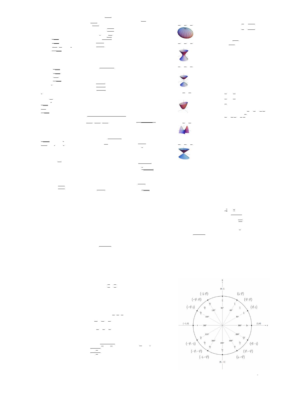
Unit Circle
(cos, sin)
Other Information
p
a
p
b
=
p
a
b
Where a Cone is defined as
z =
p
a(x
2
+ y
2
),
In Spherical Coordinates,
= cos
1
(
q
a
1+a
)
Right Circular Cylinder:
V = ⇡r
2
h, SA = ⇡r
2
+2⇡rh
lim
n!inf
(1 +
m
n
)
pn
= e
mp
Law of Cosines:
a
2
= b
2
+ c
2
2bc(cos(✓))
Stokes Th eor em
Let:
·S be a 3D surface
·
~
F (x, y , z)=
M(x, y, z)
ˆ
i + N(x, y, z)
ˆ
j + P (x, y, z)
ˆ
l
·M,N,P have continuous 1
st
order partial
derivatives
·C is piece-wise smooth, simple, closed,
curve, positively oriented
·
ˆ
T is unit tangent vector to C.
Then,
H
~
F
c
·
ˆ
TdS =
RR
s
(r⇥
~
F ) · ˆndS =
RR
R
(r⇥
~
F ) · ~ndxdy
Remember:
H
~
F ·
~
Tds =
R
c
(Mdx + Ndy + Pdz)
Originally Written By Daniel Kenner for
MATH 2210 at the University of Utah.
Source code available at
https://github.com/keytotime/Calc3 CheatSheet
Thanks to Kelly Macarthur for Teaching and
Providing Notes.