Derivatives
D
x
e
x
= e
x
D
x
sin(x)=cos(x)
D
x
cos(x)=sin(x)
D
x
tan(x)=sec
2
(x)
D
x
cot(x)=csc
2
(x)
D
x
sec(x)=sec(x)tan(x)
D
x
csc(x)=csc(x)cot(x)
D
x
sin
1
=
1
p
1x
2
,x 2 [1, 1]
D
x
cos
1
=
1
p
1x
2
,x 2 [1, 1]
D
x
tan
1
=
1
1+x
2
,
⇡
2
x
⇡
2
D
x
sec
1
=
1
|x|
p
x
2
1
, |x| > 1
D
x
sinh(x)=cosh(x)
D
x
cosh(x)=sinh(x)
D
x
tanh(x)=sech
2
(x)
D
x
coth(x)=csch
2
(x)
D
x
sech(x)=sech(x)tanh(x)
D
x
csch(x)=csch(x)coth(x)
D
x
sinh
1
=
1
p
x
2
+1
D
x
cosh
1
=
1
p
x
2
1
,x > 1
D
x
tanh
1
=
1
1x
2
1 <x<1
D
x
sech
1
=
1
x
p
1x
2
, 0 <x<1
D
x
ln(x)=
1
x
Integrals
R
1
x
dx = ln |x| + c
R
e
x
dx = e
x
+ c
R
a
x
dx =
1
ln a
a
x
+ c
R
e
ax
dx =
1
a
e
ax
+ c
R
1
p
1x
2
dx = sin
1
(x)+c
R
1
1+x
2
dx = tan
1
(x)+c
R
1
x
p
x
2
1
dx =sec
1
(x)+c
R
sinh(x)dx = cosh(x)+c
R
cosh(x)dx = sinh(x)+c
R
tanh(x)dx = ln |cosh(x)| + c
R
tanh(x)sech(x)dx = sech(x)+c
R
sech
2
(x)dx = tanh(x)+c
R
csch(x)coth(x)dx = csch(x)+c
R
tan(x)dx = ln |cos(x)| + c
R
cot(x)dx = ln |sin(x)| + c
R
cos(x)dx = sin(x)+c
R
sin(x)dx = cos(x)+c
R
1
p
a
2
u
2
dx = sin
1
(
u
a
)+c
R
1
a
2
+u
2
dx =
1
a
tan
1
u
a
+ c
R
ln(x)dx =(xln(x)) x + c
U-Substitution
Let u = f(x)(canbemorethanone
variable).
Determine: du =
f (x)
dx
dx and solve for
dx.
Then, if a definite integral, substitute
the bounds for u = f (x)ateachbounds
Solve the integral using u.
Integration by Parts
R
udv = uv
R
vdu
Fns and Identities
sin(cos
1
(x)) =
p
1 x
2
cos(sin
1
(x)) =
p
1 x
2
sec(tan
1
(x)) =
p
1+x
2
tan(sec
1
(x))
=(
p
x
2
1ifx 1)
=(
p
x
2
1 if x 1)
sinh
1
(x)=lnx +
p
x
2
+1
sinh
1
(x)=lnx +
p
x
2
1,x1
tanh
1
(x)=
1
2
ln x +
1+x
1x
, 1 <x<1
sech
1
(x)=ln[
1+
p
1x
2
x
], 0 <x1
sinh(x)=
e
x
e
x
2
cosh(x)=
e
x
+e
x
2
Trig Identities
sin
2
(x)+cos
2
(x)=1
1+tan
2
(x)=sec
2
(x)
1+cot
2
(x)=csc
2
(x)
sin(x ± y)=sin(x)cos(y) ± cos(x)sin(y)
cos(x ± y)=cos(x)cos(y) ± sin(x)sin(y)
tan(x ± y)=
tan(x)±tan(y)
1⌥tan(x) tan(y)
sin(2x)=2sin(x)cos(x)
cos(2x)=cos
2
(x) sin
2
(x)
cosh(n
2
x) sinh
2
x =1
1+tan
2
(x)=sec
2
(x)
1+cot
2
(x)=csc
2
(x)
sin
2
(x)=
1cos(2x)
2
cos
2
(x)=
1+cos(2x)
2
tan
2
(x)=
1cos(2x)
1+cos(2x)
sin(x)=sin(x)
cos(x)=cos(x)
tan(x)=tan(x)
Calculus 3 Concepts
Cartesian coords in 3D
given two p oints:
(x
1
,y
1
,z
1
)and(x
2
,y
2
,z
2
),
Distance between them:
p
(x
1
x
2
)
2
+(y
1
y
2
)
2
+(z
1
z
2
)
2
Midpoint:
(
x
1
+x
2
2
,
y
1
+y
2
2
,
z
1
+z
2
2
)
Sphere with center (h,k,l) and radius r:
(x h)
2
+(y k)
2
+(z l)
2
= r
2
Vector s
Vector : ~u
Unit Vector: ˆu
Magnitude: ||~u|| =
q
u
2
1
+ u
2
2
+ u
2
3
Unit Vector: ˆu =
~u
||~u||
Dot Product
~u · ~v
Produces a Scalar
(Geometrically, the dot product is a
vector pro jection)
~u =<u
1
,u
2
,u
3
>
~v =<v
1
,v
2
,v
3
>
~u · ~v =
~
0meansthetwovectorsare
Perpendicular ✓ is th e an gle between
them.
~u · ~v = ||~u|| ||~v|| cos(✓)
~u · ~v = u
1
v
1
+ u
2
v
2
+ u
3
v
3
NOTE:
ˆu · ˆv = cos(✓)
||~u||
2
= ~u · ~u
~u · ~v = 0 when ?
Angle Between ~u and ~v:
✓ = cos
1
(
~u·~v
||~u|| ||~v||
)
Pro jection of ~u onto ~v:
pr
~v
~u =(
~u·~v
||~v||
2
)~v
Cross Product
~u ⇥ ~v
Produces a Vector
(Geometrically, the cross product is the
area of a p aralellogram with sides ||~u||
and ||~v||)
~u =<u
1
,u
2
,u
3
>
~v =<v
1
,v
2
,v
3
>
~u ⇥ ~v =
ˆ
i
ˆ
j
ˆ
k
u
1
u
2
u
3
v
1
v
2
v
3
~u ⇥ ~v =
~
0meansthevectorsareparalell
Lines and Planes
Equation of a Plane
(x
0
,y
0
,z
0
) is a point on the plane and
<A,B,C>is a normal vector
A(x x
0
)+B(y y
0
)+C(z z
0
)=0
<A,B,C>· <xx
0
,yy
0
,zz
0
>=0
Ax + By + Cz = D where
D = Ax
0
+ By
0
+ Cz
0
Equation of a line
AlinerequiresaDirectionVector
~u =<u
1
,u
2
,u
3
> and a point
(x
1
,y
1
,z
1
)
then,
aparameterizationofalinecouldbe:
x = u
1
t + x
1
y = u
2
t + y
1
z = u
3
t + z
1
Distance from a Point to a Plane
The distance from a point (x
0
,y
0
,z
0
)to
a plane Ax+By+Cz=D can be expressed
by the formula:
d =
|Ax
0
+By
0
+Cz
0
D|
p
A
2
+B
2
+C
2
Coord Sys Conv
Cylindrical to Rectangular
x = r cos(✓)
y = r sin(✓)
z = z
Rectangular to Cylindrical
r =
p
x
2
+ y
2
tan(✓)=
y
x
z = z
Spherical to Rectangular
x = ⇢ sin()cos(✓)
y = ⇢ sin()sin(✓)
z = ⇢ cos()
Rectangular to Spherical
⇢ =
p
x
2
+ y
2
+ z
2
tan(✓)=
y
x
cos()=
z
p
x
2
+y
2
+z
2
Spherical to Cylindrical
r = ⇢ sin()
✓ = ✓
z = ⇢ cos()
Cylindrical to Spherical
⇢ =
p
r
2
+ z
2
✓ = ✓
cos()=
z
p
r
2
+z
2
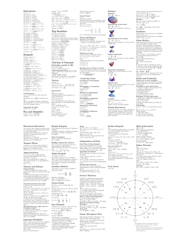
Surfaces
Ellipsoid
x
2
a
2
+
y
2
b
2
+
z
2
c
2
=1
Hyperboloid of One Sheet
x
2
a
2
+
y
2
b
2
z
2
c
2
=1
(Major Axis: z because it follows - )
Hyperboloid of Two Sheets
z
2
c
2
x
2
a
2
y
2
b
2
=1
(Major Axis: Z because it is the one not
subtracted)
Elliptic Paraboloid
z =
x
2
a
2
+
y
2
b
2
(Major Axis: z because it is the variable
NOT squared)
Hyperbolic Paraboloid
(Major Axis: Z axis because it is not
squared)
z =
y
2
b
2
x
2
a
2
Elliptic Cone
(Major Axis: Z axis because it’s the only
one being subtracted)
x
2
a
2
+
y
2
b
2
z
2
c
2
=0
Cylinder
1ofthevariablesismissing
OR
(x a)
2
+(y b
2
)=c
(Major Axis is missing variable)
Partial D er ivatives
Partial Derivatives are simply holding all
other variables constant (and act like
constants for the derivative) and only
taking the derivative with respect to a
given variable.
Given z=f(x,y), the partial derivative of
zwithrespecttoxis:
f
x
(x, y)=z
x
=
@z
@x
=
@f (x,y)
@x
likewise for partial with respect to y:
f
y
(x, y)=z
y
=
@z
@y
=
@f (x,y)
@y
Notation
For f
xyy
,work”insidetooutside”f
x
then f
xy
,thenf
xyy
f
xyy
=
@
3
f
@x@
2
y
,
For
@
3
f
@x@
2
y
,workrighttoleftinthe
denominator
Gradients
The Gradient of a function in 2 variables
is rf =<f
x
,f
y
>
The Gradient of a function in 3 variables
is rf =<f
x
,f
y
,f
z
>
Chain Rule(s)
Take the Par ti al der ivat ive wit h r es p ect
to the first-order variables of the
function times the partial (or normal)
derivative of the first-order variable to
the ultimate variable you are looking for
summed with the same process for other
first-order variables this makes sense for.
Example:
let x = x(s,t), y = y(t) and z = z (x,y).
zthenhasfirstpartialderivative:
@z
@x
and
@z
@y
xhasthepartialderivatives:
@x
@s
and
@x
@t
and y has the derivative:
dy
dt
In this case (with z containing x and y
as well as x and y b oth containing s and
t), the chain rule for
@z
@s
is
@z
@s
=
@z
@x
@x
@s
The chain rule for
@z
@t
is
@z
@t
=
@z
@x
@x
@t
+
@z
@y
dy
dt
Note: the use of ”d ” inste ad of ”@ ”with
the function of only one independent
variable
Limits and Continuity
Limits in 2 or more variables
Limits taken over a vectorized limit just
evaluate separately for each component
of the limit.
Strategies to show limit exists
1. Plug in Numbers, Everything is Fine
2. Algebraic Manipulation
-factoring/dividing out
-use trig identites
3. Change to polar coords
if(x, y) ! (0, 0) , r ! 0
Strategies to show limit DNE
1. Show limit is di↵erent if approached
from di↵erent paths
(x=y, x = y
2
, etc.)
2. Switch to Polar coords and show the
limit DNE.
Continunity
Afn,z = f (x, y), is continuous at (a,b)
if
f(a, b)=lim
(x,y)!(a,b)
f(x, y)
Which means:
1. The limit exists
2. The fn value is defined
3. They are the same value
Directional Derivatives
Let z=f(x,y) be a fuction, (a,b) ap point
in the domain (a valid input point) and
ˆu aunitvector(2D).
The Directional Derivative is then the
derivative at the point (a,b) in the
direction of ˆu or:
D
~u
f(a, b)= ˆu · rf(a, b)
This will return a scalar.4-Dversion:
D
~u
f(a, b, c)= ˆu · rf(a, b, c)
Tangent Planes
let F(x,y,z) = k be a surface and P =
(x
0
,y
0
,z
0
)beapointonthatsurface.
Equation of a Tangent Plane:
rF (x
0
,y
0
,z
0
)· <xx
0
,y y
0
,z z
0
>
Approximations
let z = f (x, y)beadi↵erentiable
function total di↵erential of f = dz
dz = rf · <dx,dy>
This is the approximate change in z
The actual change in z is the di↵erence
in z values:
z = z z
1
Maxima and Minima
Internal Points
1. Take the Partial Derivatives with
respect to X and Y (f
x
and f
y
)(Canuse
gradient)
2. Set derivatives equal to 0 and use to
solve system of equations for x and y
3. Plug back into original equation for z.
Use Second Derivative Test for whether
points are local max, min, or saddle
Second Partial Derivative Test
1. Find all ( x,y) points such that
rf(x, y)=
~
0
2. Let D = f
xx
(x, y)f
yy
(x, y) f
2
xy
(x, y)
IF (a) D > 0ANDf
xx
< 0, f(x,y) is
local max value
(b) D > 0ANDf
xx
(x, y) > 0f(x,y)is
local min value
(c) D < 0, (x,y,f(x,y)) is a saddle point
(d) D = 0, test is inconclusive
3. Determine if any boundary point
gives min or max. Typically, we have to
parametrize boundary and then reduce
to a Calc 1 type of min/max problem to
solve.
The following only apply only if a
boundary is given
1. check the corner points
2. Check each line (0 x 5would
give x=0 and x=5 )
On Bounded Equations, this is the
global min and max...second derivative
test is not needed.
Lagrange Multipliers
Given a function f(x,y) with a constraint
g(x,y), solve the following system of
equations to find the max and min
points on the constraint (NOTE: may
need to also find internal points.):
rf = rg
g(x, y)=0(orkifgiven)
Double Integrals
With Respect to the xy-axis, if taking an
integral,
RR
dydx is cutting in vertical rectangles,
RR
dxdy is cutting in horizontal
rectangles
Polar Coordinates
When using polar co ordinates,
dA = rdrd✓
Surface Area of a Curve
let z = f(x,y) be continuous over S (a
closed Region in 2D domain)
Then the surface area of z = f(x,y) over
S is:
SA =
RR
S
q
f
2
x
+ f
2
y
+1dA
Trip l e Integrals
RRR
s
f(x, y, z)dv =
R
a
2
a
1
R
2
(x)
1
(x)
R
2
(x,y)
1
(x,y)
f(x, y, z)dzdydx
Note: dv can be exchanged for dxdydz in
any order, but you must then choose
your limits of integration according to
that order
Jacobian Method
RR
G
f(g(u, v ) ,h( u, v))|J (u, v)|dudv =
RR
R
f(x, y)dxdy
J(u, v)=
@x
@u
@x
@v
@y
@u
@y
@v
Common Jacobians:
Rect. to Cylindric al: r
Rect. to Sph e rical: ⇢
2
sin()
Vector Fields
let f(x, y, z)beascalarfieldand
~
F (x, y , z)=
M(x, y, z)
ˆ
i + N(x, y, z)
ˆ
j + P (x, y, z)
ˆ
k be
avectorfield,
Grandient of f = rf =<
@f
@x
,
@f
@y
,
@f
@z
>
Divergence of
~
F :
r ·
~
F =
@M
@x
+
@N
@y
+
@P
@z
Curl of
~
F :
r⇥
~
F =
ˆ
i
ˆ
j
ˆ
k
@
@x
@
@y
@
@z
MN P
Line Integrals
Cgivenbyx = x(t),y = y(t),t 2 [a, b]
R
c
f(x, y)ds =
R
b
a
f(x(t),y(t))ds
where ds =
q
(
dx
dt
)
2
+(
dy
dt
)
2
dt
or
q
1+(
dy
dx
)
2
dx
or
q
1+(
dx
dy
)
2
dy
To eval ua te a Line Int eg ral ,
· get a p aramaterized version of the line
(usually in terms of t, though in
exclusive terms of x or y is ok)
· evaluate for the derivatives needed
(usually dy, dx, and/or dt)
· plug in to original equation to get in
terms of the independant variable
· solve integral
Wor k
Let
~
F = M
ˆ
i +
ˆ
j +
ˆ
k (force)
M = M (x, y , z),N = N ( x, y, z),P =
P (x, y, z)
(Literally)d~r = dx
ˆ
i + dy
ˆ
j + dz
ˆ
k
Work w =
R
c
~
F · d~r
(Work done by moving a particle over
curve C with force
~
F )
Independence of Path
Fun d T h m o f L in e I nt e g r a l s
Ciscurvegivenby~r(t),t 2 [a, b];
~r0(t)exists. Iff (~r)iscontinuously
di↵erentiable on an open set containing
C, then
R
c
rf(~r) · d~r = f (
~
b) f(~a)
Equivalent Conditions
~
F (~r)continuousonopenconnectedset
D. Then,
(a)
~
F = rf for some fn f. (if
~
F is
conservative)
, (b)
R
c
~
F (~r) · d~risindep.of pathinD
, (c)
R
c
~
F (~r) · d~r = 0 for all closed paths
in D.
Conservation Theorem
~
F = M
ˆ
i + N
ˆ
j + P
ˆ
k continuously
di↵erentiable on open, simply connected
set D.
~
F conservative ,r⇥
~
F =
~
0
(in 2D r⇥
~
F =
~
0i↵ M
y
= N
x
)
Green’s Theorem
(method of changing line integral for
double integral - Use for Flux and
Circulation across 2D curve and line
integrals over a closed boundary)
H
Mdy Ndx =
RR
R
(M
x
+ N
y
)dxdy
H
Mdx + Ndy =
RR
R
(N
x
M
y
)dxdy
Let:
·Rbearegioninxy-plane
·Cissimple,closedcurveenclosingR
(w/ paramerization ~r(t))
·
~
F (x, y)=M (x, y)
ˆ
i + N(x, y)
ˆ
j be
continuously di↵erentiable over R[C.
For m 1 : Fl u x A cr o ss Bo u nd a ry
~n = unit normal vector to C
H
c
~
F · ~n =
RR
R
r ·
~
FdA
,
H
Mdy Ndx =
RR
R
(M
x
+ N
y
)dxdy
For m 2 : Ci r cu l at i o n A l o n g
Boundary
H
c
~
F · d~r =
RR
R
r⇥
~
F · ˆudA
,
H
Mdx + Ndy =
RR
R
(N
x
M
y
)dxdy
Area of R
A =
H
(
1
2
ydx +
1
2
xdy)
Gauss’ Divergence Thm
(3D Analog of Green’s Theorem - Use
for Flux over a 3D surface) Let:
·
~
F (x, y , z)bevectorfieldcontinuously
di↵erentiable in solid S
·S is a 3D solid ·@S boundary of S (A
Surface)
·ˆnunit outer normal to @ S
Then,
RR
@S
~
F (x, y , z) · ˆndS =
RRR
S
r ·
~
FdV
(dV = dxdydz)
Surface Integrals
Let
·Rbeclosed,boundedregioninxy-plane
·fbeafnwithfirstorderpartial
derivatives on R
·GbeasurfaceoverRgivenby
z = f (x, y)
·g(x, y, z)=g(x, y , f (x, y)) is cont. on R
Then,
RR
G
g(x, y, z)dS =
RR
R
g(x, y, f (x, y))dS
where dS =
q
f
2
x
+ f
2
y
+1dydx
Flux of
~
F across G
RR
G
~
F · ndS =
RR
R
[Mf
x
Nf
y
+ P ]dxdy
where:
·
~
F (x, y , z)=
M(x, y, z)
ˆ
i + N(x, y, z)
ˆ
j + P (x, y, z)
ˆ
k
·G is surface f(x,y)=z
·~n is upward unit normal on G.
·f(x,y) has continuous 1
st
order partial
derivatives
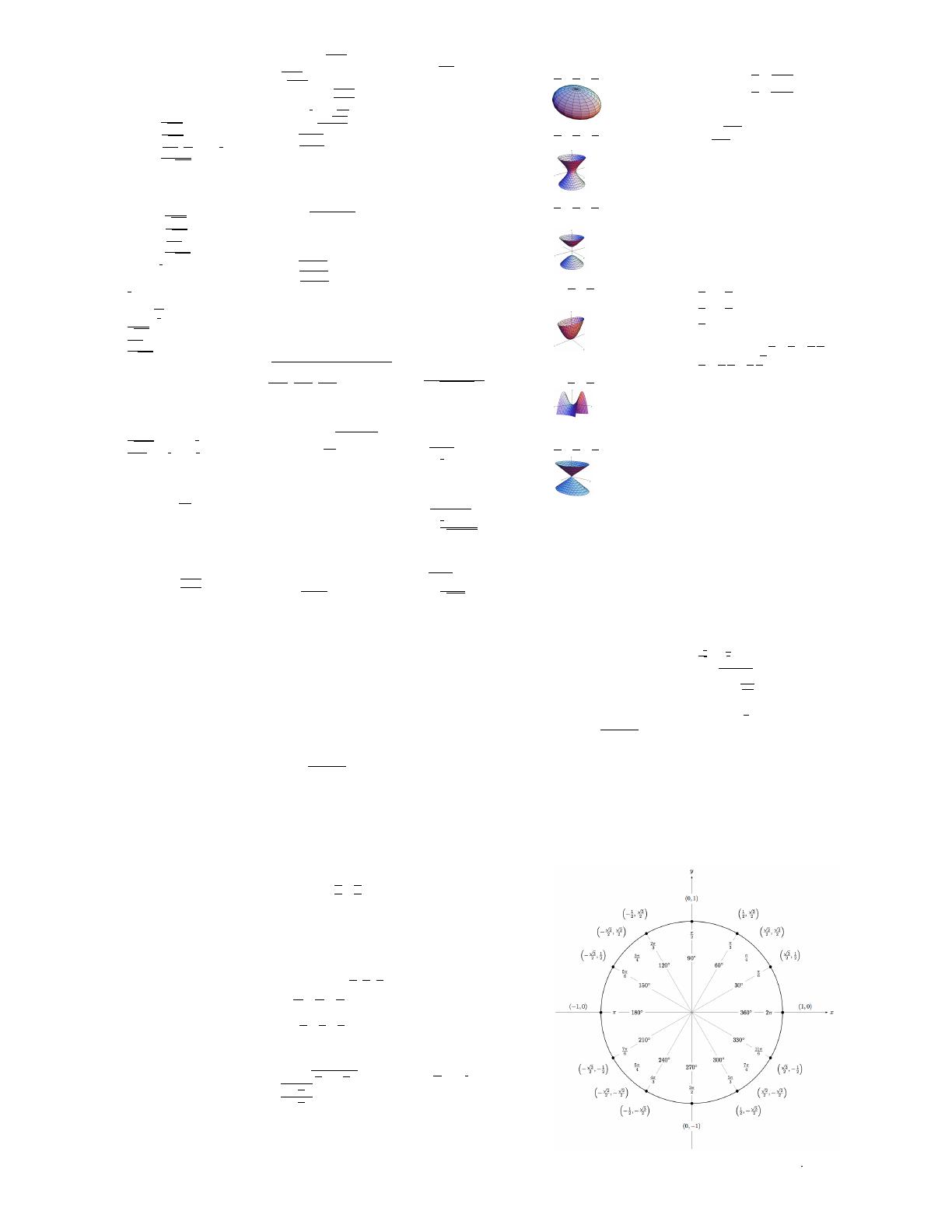
Unit Circle
(cos, sin)
Other Information
p
a
p
b
=
p
a
b
Where a Cone is defined as
z =
p
a(x
2
+ y
2
),
In Spherical Coordinates,
= cos
1
(
q
a
1+a
)
Right Circular Cylinder:
V = ⇡r
2
h, SA = ⇡r
2
+2⇡rh
lim
n!inf
(1 +
m
n
)
pn
= e
mp
Law of Cosines:
a
2
= b
2
+ c
2
2bc(cos(✓))
Stokes Th eor em
Let:
·S be a 3D surface
·
~
F (x, y , z)=
M(x, y, z)
ˆ
i + N(x, y, z)
ˆ
j + P (x, y, z)
ˆ
l
·M,N,P have continuous 1
st
order partial
derivatives
·C is piece-wise smooth, simple, closed,
curve, positively oriented
·
ˆ
T is unit tangent vector to C.
Then,
H
~
F
c
·
ˆ
TdS =
RR
s
(r⇥
~
F ) · ˆndS =
RR
R
(r⇥
~
F ) · ~ndxdy
Remember:
H
~
F ·
~
Tds =
R
c
(Mdx + Ndy + Pdz)
Originally Written By Daniel Kenner for
MATH 2210 at the University of Utah.
Source code available at
https://github.com/keytotime/Calc3 CheatSheet
Thanks to Kelly Macarthur for Teaching and
Providing Notes.