Figure 1: Examples of univariate Gaussian

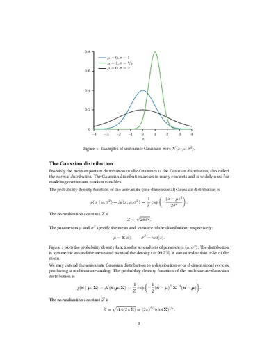
Univariate Gaussian distributions are fundamental in statistics, illustrating how continuous random variables behave. The document provides visual examples of probability density functions (PDFs) for various mean and variance parameters, showcasing the symmetric nature of the Gaussian curve. It serves as an essential resource for students and professionals studying statistical methods and probability theory. The content includes mathematical formulations and graphical representations, making it suitable for those preparing for exams in statistics or data analysis.

Key Points

Illustrates univariate Gaussian probability density functions with different parameters.
Explains the significance of mean and variance in Gaussian distributions.
Includes visual representations to aid understanding of statistical concepts.
Serves as a resource for students studying statistics and probability theory.

337

−4 −3 −2 −1 0 1 2 3 4

0.2

0.4

0.6

0.8

µ = 0, σ = 1

µ = 1, σ =

µ = 0, σ = 2

Figure 1: Examples of univariate Gaussian pdfs N(x; µ, σ

The Gaussian distribution

Probably the most-important distribution in all of statistics is the Gaussian distribution, also called

the normal distribution. The Gaussian distribution arises in many contexts and is widely used for

modeling continuous random variables.

The probability density function of the univariate (one-dimensional) Gaussian distribution is

p(x | µ, σ

) = N(x; µ, σ

) =

exp



−

(x − µ)

2σ



The normalization constant Z is

Z =

√

2πσ

The parameters µ and σ

specify the mean and variance of the distribution, respectively:

µ = E[x]; σ

= var[x].

Figure 1 plots the probability density function for several sets of parameters

(µ, σ

)

. The distribution

is symmetric around the mean and most of the density (

≈ 99.7%

) is contained within

±3σ

of the

mean.

We may extend the univariate Gaussian distribution to a distribution over

-dimensional vectors,

producing a multivariate analog. The probablity density function of the multivariate Gaussian

distribution is

p(x | µ, Σ) = N(x; µ, Σ) =

exp



−

(x − µ)

−1

(x − µ)



The normalization constant Z is

Z =

det(2πΣ) = (2π)

(det Σ)

−4 −2 0 2 4

−4

−2

(a) Σ =



1 0

0 1



−4 −2 0 2 4

−4

−2

(b) Σ =



/2 1



−4 −2 0 2 4

−4

−2



1 −1

−1 3



Figure 2: Contour plots for example bivariate Gaussian distributions. Here

µ = 0

for all examples.

Examining these equations, we can see that the multivariate density coincides with the univariate

density in the special case when Σ is the scalar σ

Again, the vector

specifies the mean of the multivariate Gaussian distribution. The matrix

specifies the covariance between each pair of variables in x:

Σ = cov(x, x) = E



(x − µ)(x − µ)



Covariance matrices are necessarily symmetric and positive semidefinite, which means their eigen-

values are nonnegative. Note that the density function above requires that

be positive definite, or

have strictly positive eigenvalues. A zero eigenvalue would result in a determinant of zero, making

the normalization impossible.

The dependence of the multivariate Gaussian density on

is entirely through the value of the

quadratic form

∆

= (x − µ)

−1

(x − µ).

The value

∆

(obtained via a square root) is called the Mahalanobis distance, and can be seen as a

generalization of the Z score

(x−µ)

, often encountered in statistics.

To understand the behavior of the density geometrically, we can set the Mahalanobis distance to a

constant. The set of points in

satisfying

∆ = c

for any given value

c > 0

is an ellipsoid with

the eigenvectors of Σ defining the directions of the principal axes.

Figure 2 shows contour plots of the density of three bivariate (two-dimensional) Gaussian distribu-

tions. The elliptical shape of the contours is clear.

The Gaussian distribution has a number of convenient analytic properties, some of which we

describe below.

Marginalization

Often we will have a set of variables

with a joint multivariate Gaussian distribution, but only be

interested in reasoning about a subset of these variables. Suppose

has a multivariate Gaussian

distribution:

p(x | µ, Σ) = N(x, µ, Σ).

−4 −2 0 2 4

−4

−2

(a) p(x | µ, Σ)

−4 −2 0 2 4

0.1

0.2

0.3

0.4

p(x

)

(b) p(x

| µ

, Σ

) = N (x

; 0, 1)

Figure 3: Marginalization example. (a) shows the joint density over

x = [x

, x

]

; this is the same

density as in Figure 2(c). (b) shows the marginal density of x

Let us partition the vector into two components:

x =





We partition the mean vector and covariance matrix in the same way:

µ =





Σ =





Now the marginal distribution of the subvector x

has a simple form:

p(x

| µ, Σ) = N(x

, µ

, Σ

so we simply pick out the entries of µ and Σ corresponding to x

Figure 3 illustrates the marginal distribution of x

for the joint distribution shown in Figure 2(c).

Conditioning

Another common scenario will be when we have a set of variables

with a joint multivariate

Gaussian prior distribution, and are then told the value of a subset of these variables. We may

then condition our prior distribution on this observation, giving a posterior distribution over the

remaining variables.

Suppose again that x has a multivariate Gaussian distribution:

p(x | µ, Σ) = N(x, µ, Σ),

and that we have partitioned as before:

x = [x

, x

]

. Suppose now that we learn the exact value

of the subvector x

. Remarkably, the posterior distribution

p(x

| x

, µ, Σ)

337

Ultimate Exercise Guide by Jeff Nippard PDF

The Miles Circuit

The Hardy Weinberg Equation Pogil

The Four Types of Symmetry in the Plane

The Basics Of Testing A Mass Air Flow (MAF) Sensor

Tcar Exam

FAQs of Figure 1: Examples of univariate Gaussian

What are the key characteristics of univariate Gaussian distributions?

Univariate Gaussian distributions are defined by their mean (µ) and variance (σ²), which determine the shape and spread of the distribution. The probability density function (PDF) is symmetric around the mean, with approximately 99.7% of the data falling within three standard deviations from the mean. This property makes the Gaussian distribution crucial for statistical analysis, as it often describes the behavior of real-valued random variables in various fields.

How does the variance affect the shape of a Gaussian distribution?

Variance in a Gaussian distribution determines the width of the curve. A smaller variance results in a steeper curve, indicating that the data points are closely clustered around the mean. Conversely, a larger variance produces a flatter curve, suggesting that the data points are more spread out. Understanding this relationship is essential for interpreting statistical data and making predictions based on Gaussian models.

What is the significance of the normalization constant in Gaussian distributions?

The normalization constant in Gaussian distributions ensures that the total area under the probability density function equals one, making it a valid probability distribution. For univariate Gaussian distributions, this constant is derived from the variance and is crucial for accurately calculating probabilities. Without this normalization, the distribution would not properly represent the likelihood of different outcomes.

What applications do univariate Gaussian distributions have in statistics?

Univariate Gaussian distributions are widely used in various statistical applications, including hypothesis testing, confidence intervals, and regression analysis. They serve as the foundation for many statistical methods, allowing researchers to model and analyze data effectively. Additionally, they are used in machine learning algorithms, where assumptions of normality can simplify complex calculations and improve model performance.